cd ..

Answering Data Science Interview Question Using Monte Carlo: Batting Average

so I saw this question a while back on twitter:

it says not to use a simulation, but we're going to use it because:

• frankly I find it easier to think literally than with abstractions

• in this day and age with the amount of processing power we have, thinking by approximations isn't obligatory anymore. and in my view the statistical pedagogy hasn't caught up to that, disservicing learners who think better with simulations

• some replies from working data scientists make me feel a bit vindicated

we'll be using Julia for its speed relative to Python. we'll also find the closed form solution after using Monte Carlo.

Monte Carlo Solution

since we're using a simulation, we can skip the Normal approximation and calculate using the original distribution, which is Binomial.

we take lots of data points from two Binomial distributions $B(45, 0.275)$ and $B(45, 0.3)$, subtract the former with the latter to get the difference, then count the probability of getting a positive batting difference.

using Distributions #stats dist. library

n = 10000 #how many times we simulate

function batting_prob_diff(n::Int)
    count( i->(i>0),
        rand(Binomial(45,0.275), n) - rand(Binomial(45,0.3), n)
        ) / n
end

it's best to display the simulation results cumulatively to see where the probabilites converge.

using Gadfly #chart library

plot(x = 1:n, 
     y = map((x) -> batting_prob_diff(x), 1:n),
     Geom.line,
     Guide.xticks(ticks=collect(0:(n/8):n)),
     Guide.yticks(ticks=collect(0:0.05:1))
)

we can see from the graph that the result approaches 0.35.

Closed Form Solution

now for the closed form solution. a Binomial distribution $B(n,p)$ can be approximated by a Normal distribution $N(np,np(1-p))$.

so the previous distributions $B(45, 0.275)$ and $B(45, 0.3)$ are approximated by $N(12.375, 8.971875)$ and $N(13.5, 9.45)$ respectively.

now, lucky for us, the distribution of the difference between two Normal distributions is also a Normal distribution.

so we'll get the resulting distribution's parameters (for Normal it's mean & variance) and calculate the probability.

the new mean is $\mu_{1}-\mu_{2} = 12.375-13.5 = -1.125$

the new variance is $\sigma_{1}^{2}+\sigma_{2}^{2} = 8.971875+9.45 = 18.421875$

we can use a cdf function in any programming language to get the solution, or use a cdf table and the z-score if you're using pen & paper (the z-score is $\frac{0-(-1.125)}{\sqrt{18.421875}} \approx -0.26$). both approaches will give you a probability of around 0.4.

Hang on a sec...

okay, something's wrong here. our closed form solution gave us 0.4, the same result Bill James got in the 70s. but our Monte Carlo simulation got us 0.35. so which one is correct?

we can start by presuming confidence in our Monte Carlo simulation, as it was a direct calculation, and cast doubt on our closed form solution which relies on approximating the original distribution into another form.

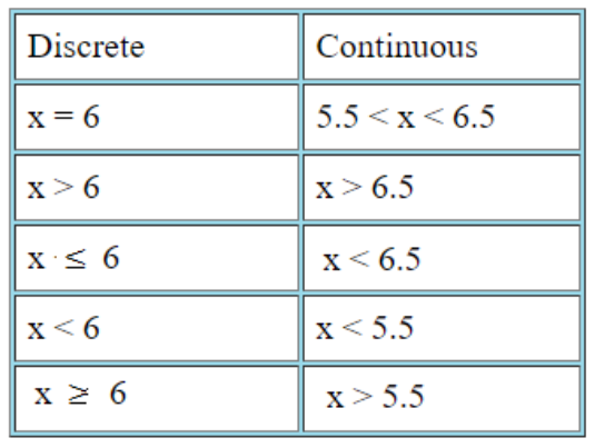
looking around online or in books, it turns out our approximation has a nontrivial issue: we estimated a discrete distribution (Binomial) with a continuous distribution (Normal), so each discrete value in the former is estimated by various values in a continuous interval from the latter.

to correct for this, we can simply subtract 0.5 from our final distribution. so instead of $P(X>0)$, we're looking for $P((X-0.5)>0) \rightarrow P(X>0.5)$.

plugging it into cdf functions or a cdf table (with the changed z-score $\frac{0.5-(-1.125)}{\sqrt{18.421875}} \approx -0.37$) gives us 0.35, the same as our Monte Carlo simulation.